Neurocomputing Part 4: Self-Organization in Artificial Neural Networks

by Simon! D. Levy

Since this issue of Extropy focuses on spontaneous order, I thought it would be appropriate to conclude my neurocomputing series with a discussion of how spontaneous orders can be modeled with neural networks. The ideas in this article were advanced primarily by Carpenter and Grossberg (1986). Lippmann (1987) provides a good summary of the Carpenter/Grossberg algorithm, along with an excellent technical outline of other neurocomputing paradigms.

One domain in which self-organization seems to play a major role is the behavior known as clustering. Clustering refers to the grouping of different objects into a single category or set of categories, based on some similarity among the objects. To take an example that we will explore here, you are able to recognize several different varieties of the letter T in print, and in handwriting, despite large differences in the appearance of the letter. Clustering represents a way of ignoring small variations in order to focus on differences that we consider significant. For this reason, neural networks that perform clustering are commonly called classifier networks.

The type of classifier network we will consider, the Carpenter/Grossberg classifier, is especially interesting from a spontaneous-orders perspective, because it learns to make classifications without supervision. All we tell it are the values of the input; the network itself determines what the outputs are. This way of learning stands in contrast to the perceptron learning algorithm and the back-propagation algorithm that I described in this series, because those two algorithms required us to tell the network what the output was supposed

to be for a given input.

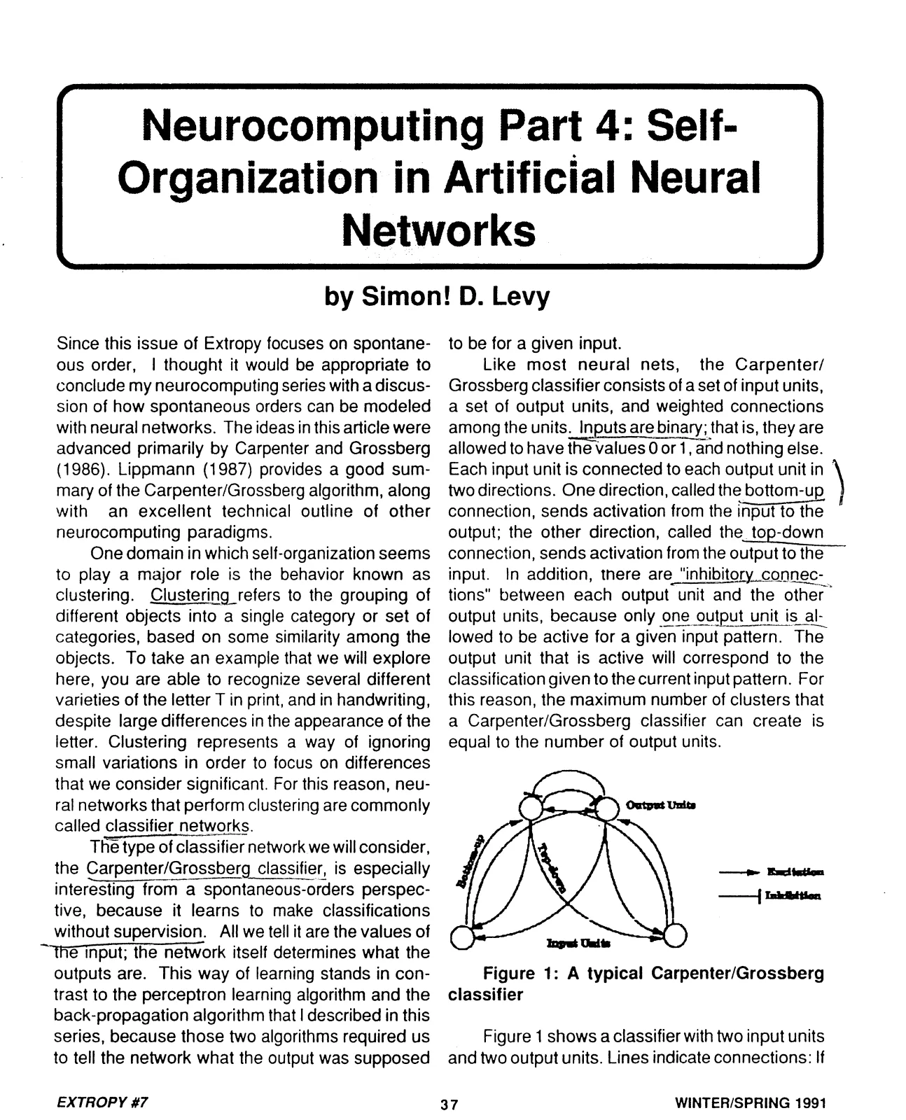
Like most neural nets, the Carpenter/Grossberg classifier consists of a set of input units, a set of output units, and weighted connections among the units. Inputs are binary; that is, they are allowed to have the values 0 or 1, and nothing else. Each input unit is connected to each output unit in two directions. One direction, called the bottom-up connection, sends activation from the input to the output; the other direction, called the top-down connection, sends activation from the output to the input. In addition, there are “inhibitory connections” between each output unit and the other output units, because only one output unit is allowed to be active for a given input pattern. The output unit that is active will correspond to the classification given to the current input pattern. For this reason, the maximum number of clusters that a Carpenter/Grossberg classifier can create is equal to the number of output units.

Figure 1: A typical Carpenter/Grossberg classifier

Figure 1 shows a classifier with two input units and two output units. Lines indicate connections: If

EXTROPY #7

37

WINTER/SPRING 1991

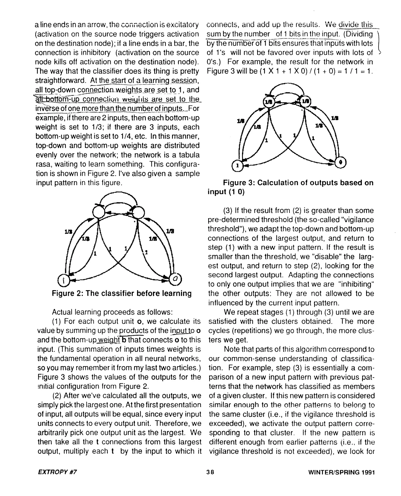
a line ends in an arrow, the connection is excitatory (activation on the source node triggers activation on the destination node); if a line ends in a bar, the connection is inhibitory (activation on the source node kills off activation on the destination node). The way that the classifier does its thing is pretty straightforward. At the start of a learning session, all top-down connection weights are set to 1, and all bottom-up connection weights are set to the inverse of one more than the number of inputs. For example, if there are 2 inputs, then each bottom-up weight is set to 1/3; if there are 3 inputs, each bottom-up weight is set to 1/4, etc. In this manner, top-down and bottom-up weights are distributed evenly over the network; the network is a tabula rasa, waiting to learn something. This configuration is shown in Figure 2. I’ve also given a sample input pattern in this figure.

Figure 2: The classifier before learning

Actual learning proceeds as follows:

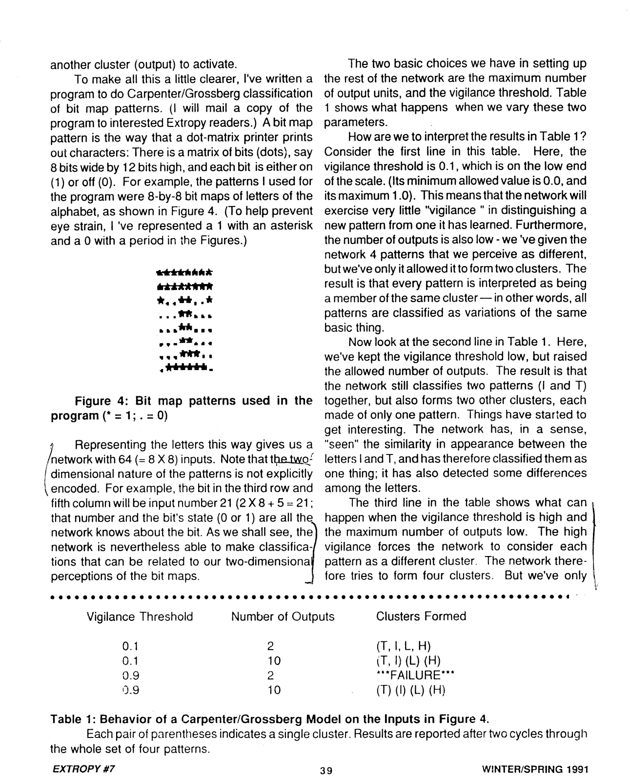
(1) For each output unit o, we calculate its value by summing up the products of the input to o and the bottom-up weight b that connects o to this input. (This summation of inputs times weights is the fundamental operation in all neural networks, so you may remember it from my last two articles.) Figure 3 shows the values of the outputs for the initial configuration from Figure 2. (2) After we’ve calculated all the outputs, we simply pick the largest one. At the first presentation of input, all outputs will be equal, since every input units connects to every output unit. Therefore, we arbitrarily pick one output unit as the largest. We then take all the t connections from this largest output, multiply each t by the input to which it

connects, and add up the results. We divide this sum by the number of 1 bits in the input. (Dividing by the number of 1 bits ensures that inputs with lots of 1’s will not be favored over inputs with lots of 0’s.) For example, the result for the network in Figure 3 will be (1 X 1 + 1 X 0) / (1 + 0) = 1 / 1 = 1.

Figure 3: Calculation of outputs based on input (1 0)

(3) If the result from (2) is greater than some pre-determined threshold (the so-called “vigilance threshold”), we adapt the top-down and bottom-up connections of the largest output, and return to step (1) with a new input pattern. If the result is smaller than the threshold, we “disable” the largest output, and return to step (2), looking for the second largest output. Adapting the connections to only one output implies that we are “inhibiting” the other outputs: They are not allowed to be influenced by the current input pattern.

We repeat stages (1) through (3) until we are satisfied with the clusters obtained. The more cycles (repetitions) we go through, the more clusters we get.

Note that parts of this algorithm correspond to our common-sense understanding of classification. For example, step (3) is essentially a comparison of a new input pattern with previous patterns that the network has classified as members of a given cluster. If this new pattern is considered similar enough to the other patterns to belong to the same cluster (i.e., if the vigilance threshold is exceeded), we activate the output pattern corresponding to that cluster. If the new pattern is different enough from earlier patterns (i.e., if the vigilance threshold is not exceeded), we look for

EXTROPY #7

38

WINTER/SPRING 1991

another cluster (output) to activate.

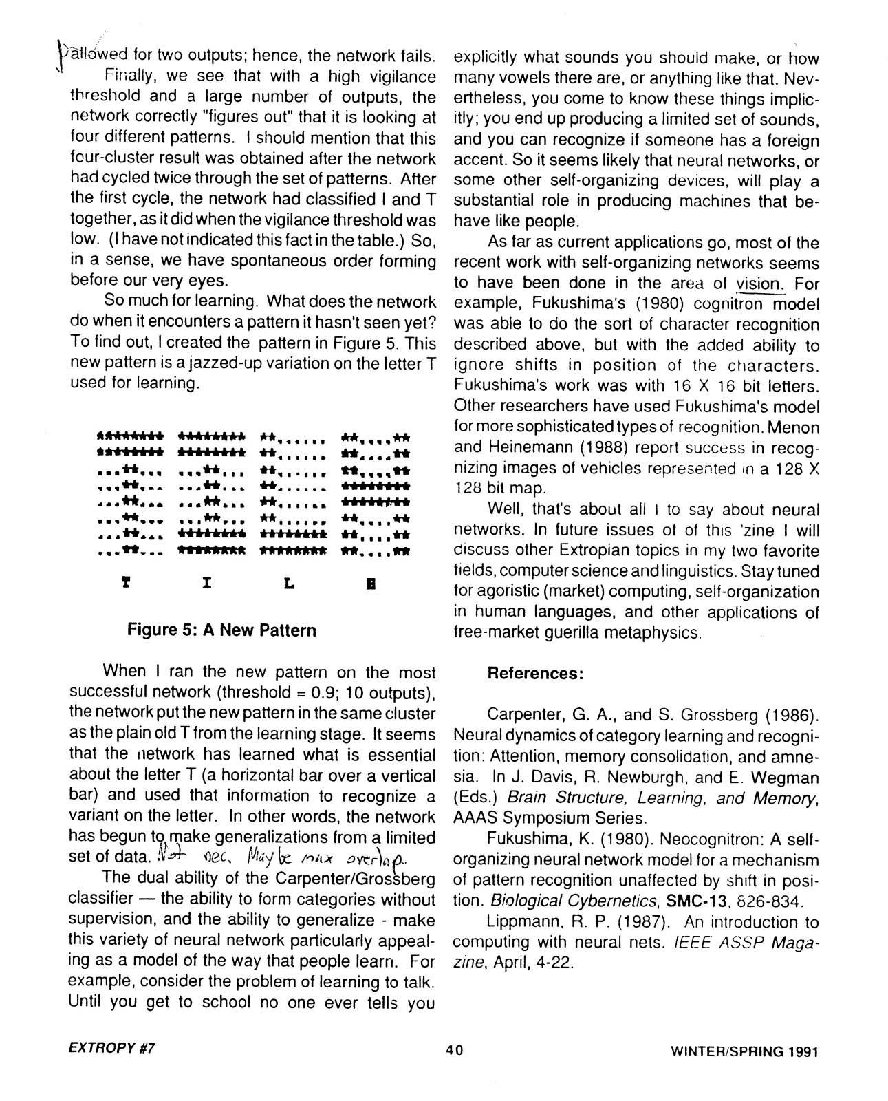
To make all this a little clearer, I’ve written a program to do Carpenter/Grossberg classification of bit map patterns. (I will mail a copy of the program to interested Extropy readers.) A bit map pattern is the way that a dot-matrix printer prints out characters: There is a matrix of bits (dots), say 8 bits wide by 12 bits high, and each bit is either on (1) or off (0). For example, the patterns I used for the program were 8-by-8 bit maps of letters of the alphabet, as shown in Figure 4. (To help prevent eye strain, I’ve represented a 1 with an asterisk and a 0 with a period in the Figures.)

Figure 4: Bit map patterns used in the program (* = 1; . = 0)

Representing the letters this way gives us a network with 64 (= 8 X 8) inputs. Note that the two-dimensional nature of the patterns is not explicitly encoded. For example, the bit in the third row and fifth column will be input number 21 (2 X 8 + 5 = 21; that number and the bit’s state (0 or 1) are all the network knows about the bit. As we shall see, the network is nevertheless able to make classifications that can be related to our two-dimensional perceptions of the bit maps.

The two basic choices we have in setting up the rest of the network are the maximum number of output units, and the vigilance threshold. Table 1 shows what happens when we vary these two parameters.

How are we to interpret the results in Table 1? Consider the first line in this table. Here, the vigilance threshold is 0.1, which is on the low end of the scale. (Its minimum allowed value is 0.0, and its maximum 1.0). This means that the network will exercise very little “vigilance” in distinguishing a new pattern from one it has learned. Furthermore, the number of outputs is also low - we’ve given the network 4 patterns that we perceive as different, but we’ve only it allowed it to form two clusters. The result is that every pattern is interpreted as being a member of the same cluster — in other words, all patterns are classified as variations of the same basic thing.

Now look at the second line in Table 1. Here, we’ve kept the vigilance threshold low, but raised the allowed number of outputs. The result is that the network still classifies two patterns (I and T) together, but also forms two other clusters, each made of only one pattern. Things have started to get interesting. The network has, in a sense, “seen” the similarity in appearance between the letters I and T, and has therefore classified them as one thing; it has also detected some differences among the letters.

The third line in the table shows what can happen when the vigilance threshold is high and the maximum number of outputs low. The high vigilance forces the network to consider each pattern as a different cluster. The network therefore tries to form four clusters. But we’ve only

Vigilance Threshold	Number of Outputs	Clusters Formed
0.1	2	(T, I, L, H)
0.1	10	(T, I) (L) (H)
0.9	2	FAILURE
0.9	10	(T) (I) (L) (H)

Table 1: Behavior of a Carpenter/Grossberg Model on the Inputs in Figure 4.

Each pair of parentheses indicates a single cluster. Results are reported after two cycles through the whole set of four patterns.

EXTROPY #7

39

WINTER/SPRING 1991

allowed for two outputs; hence, the network fails.

Finally, we see that with a high vigilance threshold and a large number of outputs, the network correctly “figures out” that it is looking at four different patterns. I should mention that this four-cluster result was obtained after the network had cycled twice through the set of patterns. After the first cycle, the network had classified I and T together, as it did when the vigilance threshold was low. (I have not indicated this fact in the table.) So, in a sense, we have spontaneous order forming before our very eyes.

So much for learning. What does the network do when it encounters a pattern it hasn’t seen yet? To find out, I created the pattern in Figure 5. This new pattern is a jazzed-up variation on the letter T used for learning.

Figure 5: A New Pattern

When I ran the new pattern on the most successful network (threshold = 0.9; 10 outputs), the network put the new pattern in the same cluster as the plain old T from the learning stage. It seems that the network has learned what is essential about the letter T (a horizontal bar over a vertical bar) and used that information to recognize a variant on the letter. In other words, the network has begun to make generalizations from a limited set of data. Not nec. Maybe max overlap.

The dual ability of the Carpenter/Grossberg classifier — the ability to form categories without supervision, and the ability to generalize - make this variety of neural network particularly appealing as a model of the way that people learn. For example, consider the problem of learning to talk. Until you get to school no one ever tells you

explicitly what sounds you should make, or how many vowels there are, or anything like that. Nevertheless, you come to know these things implicitly; you end up producing a limited set of sounds, and you can recognize if someone has a foreign accent. So it seems likely that neural networks, or some other self-organizing devices, will play a substantial role in producing machines that behave like people.

As far as current applications go, most of the recent work with self-organizing networks seems to have been done in the area of vision. For example, Fukushima’s (1980) cognitron model was able to do the sort of character recognition described above, but with the added ability to ignore shifts in position of the characters. Fukushima’s work was with 16 X 16 bit letters. Other researchers have used Fukushima’s model for more sophisticated types of recognition. Menon and Heinemann (1988) report success in recognizing images of vehicles represented in a 128 X 128 bit map.

Well, that’s about all I to say about neural networks. In future issues of of this ‘zine I will discuss other Extropian topics in my two favorite fields, computer science and linguistics. Stay tuned for agoristic (market) computing, self-organization in human languages, and other applications of free-market guerilla metaphysics.

References:

Carpenter, G. A., and S. Grossberg (1986). Neural dynamics of category learning and recognition: Attention, memory consolidation, and amnesia. In J. Davis, R. Newburgh, and E. Wegman (Eds.) Brain Structure, Learning, and Memory, AAAS Symposium Series.

Fukushima, K. (1980). Neocognitron: A self-organizing neural network model for a mechanism of pattern recognition unaffected by shift in position. Biological Cybernetics, SMC-13, 826-834.

Lippmann, R. P. (1987). An introduction to computing with neural nets. IEEE ASSP Magazine, April, 4-22.

EXTROPY #7

40

WINTER/SPRING 1991