Neurocomputing 7:

Sequential Networks

and their Dynamics

by Simon! D. Levy

In the last two installments of this series, I departed a bit from the neural networks theme to give readers a taste of some exciting developments in related fields. In this issue of Extropy I return to neural networks in order to describe a relatively new type of net that is the focus of a great deal of current research in connectionist modeling, namely, sequential (a.k.a. recurrent) neural networks.

Recall that the basic task of a neural network is to perform a mapping between two sets of data patterns, usually referred to as the input and output patterns. In the exclusive-OR (XOR) network that I have used as an example in this series, the patterns consist of binary digits (ones and zeros); the input patterns consist of pairs of these digits, and the output patterns of a single digit. The goal in the XOR problem is to “train” the network to produce an output of one when the members of the input pair are different from each other, and a zero when they are the same.

The most general thing that can be said about such a network is that it will always produce the same output pattern every time you present it with a given input pattern. If we present a well-trained XOR network five times with the pattern (0,1), it will spit out five 1’s.

connections into a neural net, we can provide this type of feedback mechanism. One nice result is that the network can now learn not just static patterns, but patterns made of se-

quences, which is why these sorts of networks are usually referred to as “sequential” or “recurrent” nets.

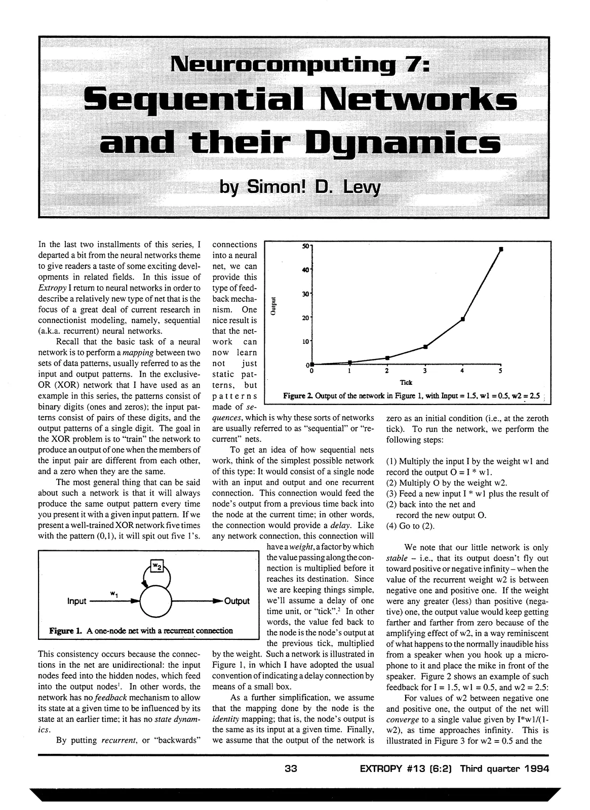
To get an idea of how sequential nets work, think of the simplest possible network of this type: It would consist of a single node with an input and output and one recurrent connection. This connection would feed the node’s output from a previous time back into the node at the current time; in other words, the connection would provide a delay. Like any network connection, this connection will

Figure 2. Output of the network in Figure 1, with Input = 1.5, w1 = 0.5, w2 = 2.5

zero as an initial condition (i.e., at the zeroth tick). To run the network, we perform the following steps:

(1) Multiply the input I by the weight w1 and record the output ( \mathrm{O} = \mathrm{I} * \mathrm{w}1 ). (2) Multiply O by the weight w2. (3) Feed a new input ( \mathrm{I} * \mathrm{w}1 ) plus the result of (2) back into the net and record the new output O. (4) Go to (2).

Figure 1. A one-node net with a recurrent connection

This consistency occurs because the connections in the net are unidirectional: the input nodes feed into the hidden nodes, which feed into the output nodes¹. In other words, the network has no feedback mechanism to allow its state at a given time to be influenced by its state at an earlier time; it has no state dynamics.

By putting recurrent, or “backwards”

have a weight, a factor by which the value passing along the connection is multiplied before it reaches its destination. Since we are keeping things simple, we’ll assume a delay of one time unit, or “tick”.² In other words, the value fed back to the node is the node’s output at the previous tick, multiplied

by the weight. Such a network is illustrated in Figure 1, in which I have adopted the usual convention of indicating a delay connection by means of a small box.

As a further simplification, we assume that the mapping done by the node is the identity mapping; that is, the node’s output is the same as its input at a given time. Finally, we assume that the output of the network is

We note that our little network is only stable - i.e., that its output doesn’t fly out toward positive or negative infinity - when the value of the recurrent weight w2 is between negative one and positive one. If the weight were any greater (less) than positive (negative) one, the output value would keep getting farther and farther from zero because of the amplifying effect of w2, in a way reminiscent of what happens to the normally inaudible hiss from a speaker when you hook up a microphone to it and place the mike in front of the speaker. Figure 2 shows an example of such feedback for I = 1.5, w1 = 0.5, and w2 = 2.5:

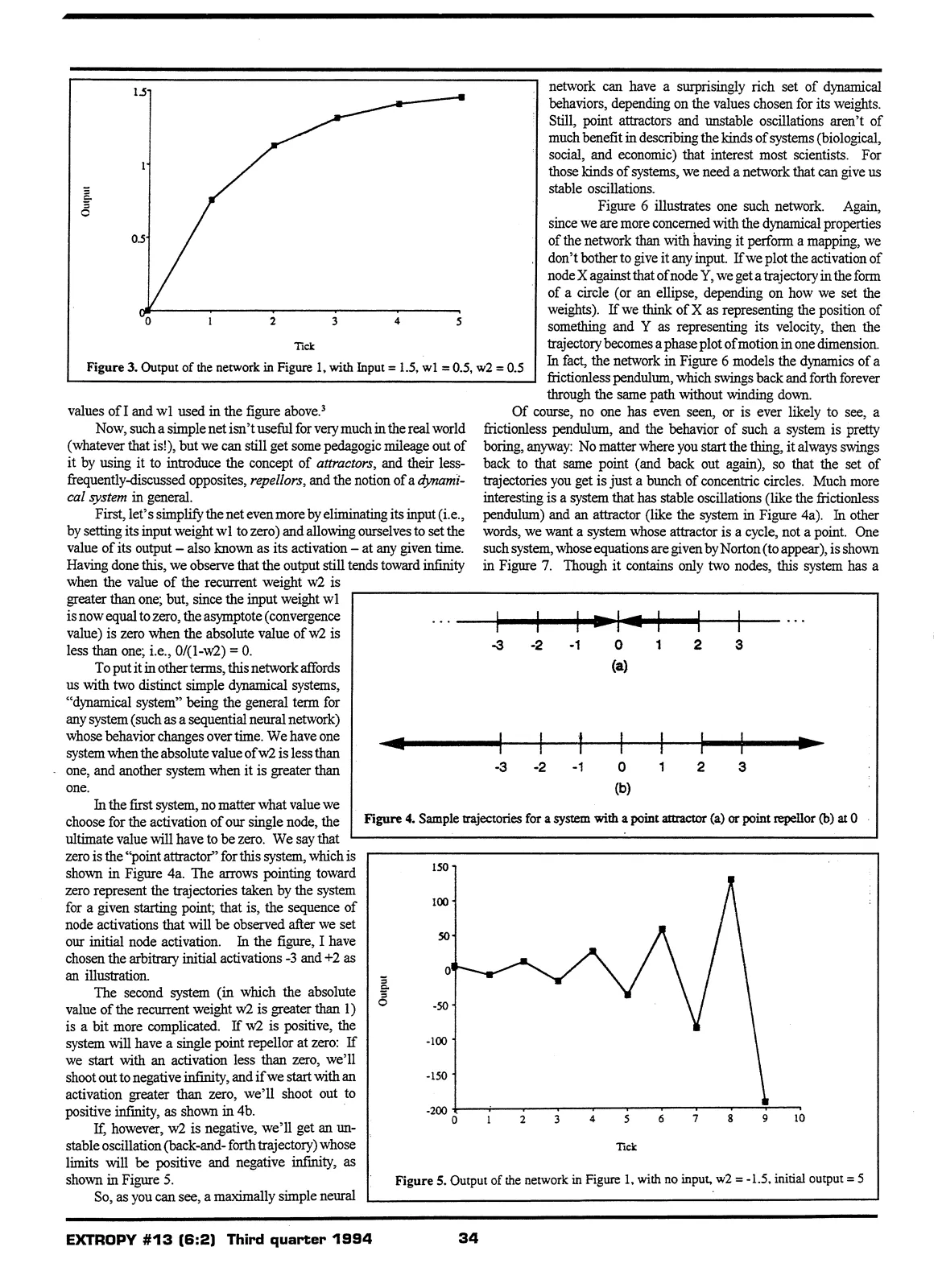
For values of w2 between negative one and positive one, the output of the net will converge to a single value given by I*w1/(1-w2), as time approaches infinity. This is illustrated in Figure 3 for w2 = 0.5 and the

33

EXTROPY #13 (6:2) Third quarter 1994

values of I and w1 used in the figure above.³

Now, such a simple net isn’t useful for very much in the real world (whatever that is!), but we can still get some pedagogic mileage out of it by using it to introduce the concept of attractors, and their less-frequently-discussed opposites, repellors, and the notion of a dynamical system in general.

First, let’s simplify the net even more by eliminating its input (i.e., by setting its input weight w1 to zero) and allowing ourselves to set the value of its output – also known as its activation – at any given time. Having done this, we observe that the output still tends toward infinity

when the value of the recurrent weight w2 is greater than one; but, since the input weight w1 is now equal to zero, the asymptote (convergence value) is zero when the absolute value of w2 is less than one; i.e., 0/(1-w2) = 0.

To put it in other terms, this network affords us with two distinct simple dynamical systems, “dynamical system” being the general term for any system (such as a sequential neural network) whose behavior changes over time. We have one system when the absolute value of w2 is less than one, and another system when it is greater than one.

In the first system, no matter what value we choose for the activation of our single node, the ultimate value will have to be zero. We say that zero is the “point attractor” for this system, which is shown in Figure 4a. The arrows pointing toward zero represent the trajectories taken by the system for a given starting point; that is, the sequence of node activations that will be observed after we set our initial node activation. In the figure, I have chosen the arbitrary initial activations -3 and +2 as an illustration.

The second system (in which the absolute value of the recurrent weight w2 is greater than 1) is a bit more complicated. If w2 is positive, the system will have a single point repellor at zero: If we start with an activation less than zero, we’ll shoot out to negative infinity, and if we start with an activation greater than zero, we’ll shoot out to positive infinity, as shown in 4b.

If, however, w2 is negative, we’ll get an unstable oscillation (back-and- forth trajectory) whose limits will be positive and negative infinity, as shown in Figure 5.

So, as you can see, a maximally simple neural

network can have a surprisingly rich set of dynamical behaviors, depending on the values chosen for its weights. Still, point attractors and unstable oscillations aren’t of much benefit in describing the kinds of systems (biological, social, and economic) that interest most scientists. For those kinds of systems, we need a network that can give us stable oscillations.

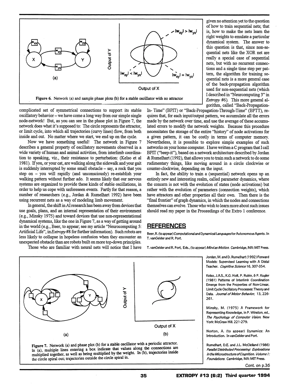
Figure 6 illustrates one such network. Again, since we are more concerned with the dynamical properties of the network than with having it perform a mapping, we don’t bother to give it any input. If we plot the activation of node X against that of node Y, we get a trajectory in the form of a circle (or an ellipse, depending on how we set the weights). If we think of X as representing the position of something and Y as representing its velocity, then the trajectory becomes a phase plot of motion in one dimension. In fact, the network in Figure 6 models the dynamics of a frictionless pendulum, which swings back and forth forever through the same path without winding down.

Of course, no one has even seen, or is ever likely to see, a frictionless pendulum, and the behavior of such a system is pretty boring, anyway: No matter where you start the thing, it always swings back to that same point (and back out again), so that the set of trajectories you get is just a bunch of concentric circles. Much more interesting is a system that has stable oscillations (like the frictionless pendulum) and an attractor (like the system in Figure 4a). In other words, we want a system whose attractor is a cycle, not a point. One such system, whose equations are given by Norton (to appear), is shown in Figure 7. Though it contains only two nodes, this system has a

Figure 4. Sample trajectories for a system with a point attractor (a) or point repellor (b) at 0

Figure 5. Output of the network in Figure 1, with no input, w2 = -1.5, initial output = 5

EXTROPY #13 (6:2) Third quarter 1994

34

(a)

Output of X

Figure 6. Network (a) and sample phase plots (b) for a stable oscillator with no attractor

given no attention yet to the question of how to train sequential nets; that is, how to make the nets learn the right weights to emulate a particular dynamical system. The answer to this question is that, since non-sequential nets like the XOR net are really a special case of sequential nets, but with no recurrent connections and a single time step per pattern, the algorithm for training sequential nets is a more general case of the back-propagation algorithm used for non-sequential nets (which I described in “Neurocomputing 3” in Extropy #6). This more general algorithm, called “Back-Propagation-

complicated set of symmetrical connections to support its stable oscillatory behavior – we have come a long way from our simple single node-network! But, as you can see in the phase plot in Figure 7, the network does what it’s supposed to: The circle represents the attractor, or limit cycle, into which all trajectories (curvy lines) flow, from both inside and out. No matter where we start, we end up on the cycle.

Now we have something useful! The network in Figure 7 describes a general property of oscillatory movements observed in a wide variety of human and animal activities, from interlimb coordination to speaking, viz., their resistance to perturbation: (Kelso et al 1981). If you, or your cat, are walking along the sidewalk and your gait is suddenly interrupted by some small obstacle – say, a rock that you step on – you will rapidly (and unconsciously) re-establish your walking pattern without further ado. It seems likely that our nervous systems are organized to provide these kinds of stable oscillations, in order to help us cope with unforeseen events. Partly for that reason, a number of researchers (e.g., Jordan & Rumelhart 1992) have been using recurrent nets as a way of modeling limb movement.

In general, the shift in AI research has been away from devices that use goals, plans, and an internal representation of their environment (e.g., Minsky 1975) and toward devices that use non-representational dynamical systems, like the one in Figure 7, as a way of getting around in the world (e.g., Beer, to appear; see my article “Neurocomputing 5: Artificial Life”, in Extropy #8 for further information). Such robots are less likely to collapse in hopeless confusion when they encounter an unexpected obstacle than are robots built on more top-down principles.

Those who are familiar with neural nets will notice that I have

In-Time” (BPIT) or “Back-Propagation-Through-Time” (BPTT), requires that, for each input/output pattern, we accumulate all the errors made by the network over time, and use the average of these accumulated errors to modify the network weights. Because this procedure necessitates the storage of the entire “history” of node activations for a given pattern, it can be costly in terms of computer memory. Nevertheless, it is possible to explore simple examples of such networks on your home computer. I have written a C program that I call BPIT (“beep-it”), based on a network architecture described by Jordan & Rumelhart (1992), that allows you to train such a network to do some rudimentary things, like moving around in a circle clockwise or counter-clockwise, depending on the input.

In fact, the ability to train a (sequential) network opens up an entirely new and interesting realm, called parameter dynamics, where the concern is not with the evolution of states (node activations) but rather with the evolution of parameters (connection weights), which have attractors and other properties all their own. Then there is the “final frontier” of graph dynamics, in which the nodes and connections themselves can evolve. Those who wish to learn more about such issues should read my paper in the Proceedings of the Extro 1 conference.

REFERENCES

Beer, R. (to appear) Computational and Dynamical Languages for Autonomous Agents. In T. vanGelder and R. Port.

T. vanGelder and R. Port, Eds., (to appear) Mind as Motion. Cambridge, MA: MIT Press.

(a)

Output of Y

Output of X

(b)

Figure 7. Network (a) and phase plot (b) for a stable oscillator with a periodic attractor. In (a), multiple lines entering a box indicate that values along the connections are multiplied together, as well as being multiplied by the weight. In (b), trajectories inside the circle spiral out; trajectories outside the circle spiral in.

Jordan, M. and D. Rumelhart (1992) Forward Models: Supervised Learning with A Distal Teacher. Cognitive Science 16, 307-354.

Kelso, J.A.S., K.G. Holt, P. Rubin, & P. Kugler (1981) Patterns of Interlimb Coordination Emerge from the Properties of Non-Linear, Limit Cycle Oscillatory Processes: Theory and Data. Journal of Motor Behavior, 13, 226-261.

Minsky, M. (1975) A Framework for Representing Knowledge, in P. Winston, ed., The Psychology of Computer Vision. New York: McGraw Hill. 221-279.

Norton, A. (to appear) Dynamics: An Introduction. In vanGelder and Port.

Rumelhart, D.E. and J.L. McClelland (1986) Parallel Distributed Processing: Explorations in the Microstructure of Cognition. Volume I: Foundations. Cambridge, MA: MIT Press.

Cont. on p.36

35

EXTROPY #13 (6:2) Third quarter 1994