-----BEGIN EXTROPY ARTICLE-----
Issue: EXTROPY #10 · Winter/Spring 1993
Author: J. Storrs Hall
Pages: 29–35 · 7 scanned pages

Nanocomputers: 21st Century Hypercomputing

by J. Storrs Hall

21st Century hypercomputing

J. Storrs Hall

If the price and performance figures for transportation technology had followed the same curves as those for computers for the past 50 years, you’d be able to buy a top-of-the-line luxury car for $10. What’s more, its mileage would be such as to allow you to drive around the world on one gallon of gas. That would only take about half an hour since top speed would be in the neighborhood of 50,000 mph (twice Earth’s escape velocity).

Oh, yes, and it would seat 5000 people.

Comparisons like this serve to point out just how radically computers have improved in cost, power consumption, speed, and memory capacity over the past half century. Is it possible that we could see as much improvement again, and in less than another half century? The answer appears to be yes.

At one time, people measured the technological sophistication of computers in ‘generations’. There were vacuum tubes, discrete transistors, IC’s, and finally large scale integration. However, since the mid-70’s, the entire processing unit has increasingly come to be put on a single chip and called a ‘microprocessor.’ After these future advances have happened, today’s microprocessors will look the way ENIAC does to us now. The then-extant computers need a different name; we’ll refer to them as nanocomputers. ‘Micro’ does exemplify at least the device size (on the order of a micron) and instruction speed (on the order of a microsecond) of the microprocessor. In at least one design, which we’ll examine below, the nanometer and nanosecond are the appropriate measures instead.

Do we really need nanocomputers? After all, you have to be able to see the screen and press the keys even if the processor is microscopic. The answer to this question lies in realizing just how closely economics and technological constraints determine what computers are used for. In the mid-sixties, IBM sold a small computer for what was then the average price

of a house. Today, single-chip micros of roughly the same computational power cost less than $5 and are used as controllers in toaster-ovens. Similarly, we can imagine putting a nanocomputer in each particle of pigment to implement ‘intelligent paint’, or at each pixel location in an artificial retina to implement image understanding algorithms.

This last is a point worth emphasizing. With today’s processing technology, robots operating outside a rigid, tightly controlled environment are extremely expensive and running at the ragged edge of the state of the art. Even though current systems can, for example, drive in traffic at highway speeds, no one is going to replace truck drivers with them until their cost comes down by some orders of magnitude. Effective robotics depends on enough computational power to perform sensory perception; nanocomputers should make this cost-effective the way microcomputers did text processing.

Beyond providing robots with the processing power humans already have, there is the opportunity of extending those powers themselves. Nanocomputers represent enough power in little enough space that it would make sense to implant them in your head to extend your sensorium, augment your memory, sharpen your reasoning. As is slowly being understood in the world of existing computers, the interface to the human is easily the most computationally intensive task of all.

Last but not least – in some sense, the most important application for nanocomputers – is as the controllers for nanomechanical devices. In particular, molecular assemblers will need nanocomputers to control them; and we will need assemblers to build nanocomputers. (In the jargon of nanotechnology, an ‘assembler’ is a robot or other mechanical manipulator small enough to build objects using tools and building blocks that are individual molecules.)

What is a nanocomputer?

Currently, the feature sizes in state-of-the-art VLSI fabrication are on the order of half a micron, i.e. 500 nanometers. In fifteen years, using nothing more than a curve-fitting, trend-line prediction, this number will be somewhere in the neighborhood of 10 nanometers; would it be appropriate to refer to such a chip as a nanocomputer?

For the purposes of this article, no. We want to talk about much more specific notions of future computing technology. First, we’re expecting the thing to be built with atomic precision. This does not mean that there will be some robot arm that places one atom, then another, and so forth, until the whole computer is done. It means that the ‘design’ of the computer specifies where each atom is to be. We expect the working parts (whether electrical or mechanical) to be essentially single molecules.

We can reasonably expect the switches, gates, or other embodiment of the logical elements to be on the order of a nanometer in size. (They may have to be further apart than that if electrical, due to electron tunneling.) In any case, it is quite reasonable to expect the entire computer to be smaller than a cubic micron, which contains a billion cubic nanometers.

Nanotechnology

The nanotechnology-assembler-nanocomputer dependence sounds like a self-referential loop, and it is. But many technologies are that way; machine tools make precision parts used in machine tools. Bootstrapping into a self-supporting technology is not a trivial problem, but it’s not an impossible one either.

Another self-referential loop in nanotechnology is slightly more complicated. We would like assemblers to be self-reproducing. This would allow for nanocomputers and other nanotechnological products to be inexpensive, be-

EXTROPY #10 Winter/Spring 1993

cause each fixed initial investment would lead to an exponentially increasing number of nanomechanisms, rather than a linearly increasing number.

But how can a machine make a copy of itself? The problem is that while we can imagine, for example, a robot arm that can screw, bolt, solder, and weld enough to assemble a robot arm from parts, it needs a sequence of instructions to obey in this process. And there is more than one instruction per part. But the instructions must be embodied in some physical form, so to finish the process, we need

General computer principles

When you get right down to it, a computer is just a device for changing information. You put in your input, and it gives you your output. If it’s being used as the controller for anything from a toaster to a robot, it gets its input from its sensors and gives its output to its motors, switches, solenoids, speakers, and what have you.

Internally, the computer has a memory, which is used to store the information it’s working on. Many functions, even so simple as a push-on, push-off

computer, then, we need some way to remember bits; some way to perform boolean logic; and some way to clock the sequence of remember, perform, remember, perform, etc.

In computers from historical times to date, information has been encoded either as the position of a mechanical part, the voltage on a wire, or a combination (as in a relay-based computer). The major reason is that these are the easiest encodings to use in the logic part of the particular technology in question. It seems reasonable to expect to see these encodings at the nano level, for the same reasons.

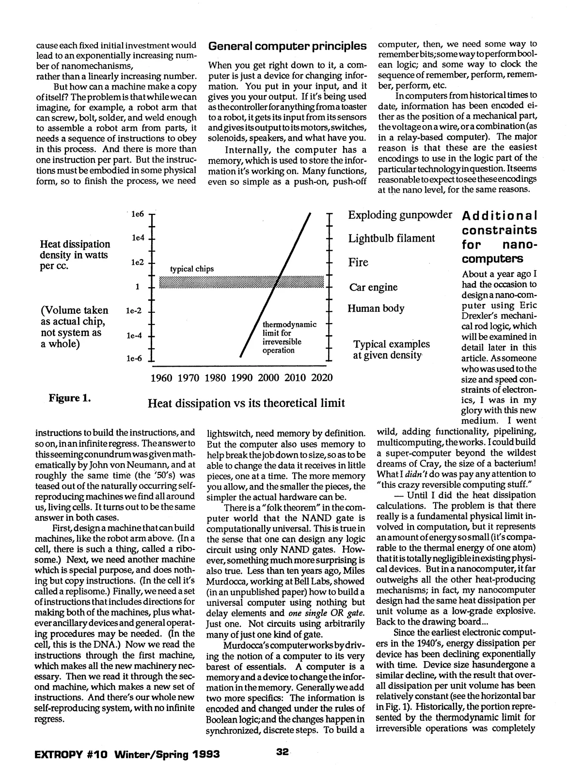
Heat dissipation density in watts per cc.

(Volume taken as actual chip, not system as a whole)

Figure 1.

Heat dissipation vs its theoretical limit

Exploding gunpowder

Lightbulb filament

Fire

Car engine

Human body

Typical examples at given density

Additional constraints for nano-computers

About a year ago I had the occasion to design a nano-computer using Eric Drexler’s mechanical rod logic, which will be examined in detail later in this article. As someone who was used to the size and speed constraints of electronics, I was in my glory with this new medium. I went

instructions to build the instructions, and so on, in an infinite regress. The answer to this seeming conundrum was given mathematically by John von Neumann, and at roughly the same time (the ‘50’s) was teased out of the naturally occurring self-reproducing machines we find all around us, living cells. It turns out to be the same answer in both cases.

First, design a machine that can build machines, like the robot arm above. (In a cell, there is such a thing, called a ribosome.) Next, we need another machine which is special purpose, and does nothing but copy instructions. (In the cell it’s called a replisome.) Finally, we need a set of instructions that includes directions for making both of the machines, plus whatever ancillary devices and general operating procedures may be needed. (In the cell, this is the DNA.) Now we read the instructions through the first machine, which makes all the new machinery necessary. Then we read it through the second machine, which makes a new set of instructions. And there’s our whole new self-reproducing system, with no infinite regress.

lightswitch, need memory by definition. But the computer also uses memory to help break the job down to size, so as to be able to change the data it receives in little pieces, one at a time. The more memory you allow, and the smaller the pieces, the simpler the actual hardware can be.

There is a “folk theorem” in the computer world that the NAND gate is computationally universal. This is true in the sense that one can design any logic circuit using only NAND gates. However, something much more surprising is also true. Less than ten years ago, Miles Murdocca, working at Bell Labs, showed (in an unpublished paper) how to build a universal computer using nothing but delay elements and one single OR gate. Just one. Not circuits using arbitrarily many of just one kind of gate.

Murdocca’s computer works by driving the notion of a computer to its very barest of essentials. A computer is a memory and a device to change the information in the memory. Generally we add two more specifics: The information is encoded and changed under the rules of Boolean logic; and the changes happen in synchronized, discrete steps. To build a

wild, adding functionality, pipelining, multicomputing, the works. I could build a super-computer beyond the wildest dreams of Cray, the size of a bacterium! What I didn’t do was pay any attention to “this crazy reversible computing stuff.”

— Until I did the heat dissipation calculations. The problem is that there really is a fundamental physical limit involved in computation, but it represents an amount of energy so small (it’s comparable to the thermal energy of one atom) that it is totally negligible in existing physical devices. But in a nanocomputer, it far outweighs all the other heat-producing mechanisms; in fact, my nanocomputer design had the same heat dissipation per unit volume as a low-grade explosive. Back to the drawing board…

Since the earliest electronic computers in the 1940’s, energy dissipation per device has been declining exponentially with time. Device size has undergone a similar decline, with the result that overall dissipation per unit volume has been relatively constant (see the horizontal bar in Fig. 1). Historically, the portion represented by the thermodynamic limit for irreversible operations was completely

EXTROPY #10 Winter/Spring 1993

insignificant; it is still in the parts per million range. However, with densities and speeds in the expected range for nanocomputers, it is extremely significant. Thus nanocomputer designers will be forced to pay attention to reversibility.

Efficient computers, like efficient heat engines, must be as nearly reversible as possible. Rolf Landauer showed in a landmark paper (in 1961) that the characteristic irreversible operation in computation is the erasure of a bit of information; the other operations can be carried out in principle reversibly and without the dissipation of energy. And as in heat engines, the reason reversibility matters is the Second Law of Thermodynamics, the law of entropy.

Entropy

The subject of entropy seems to give rise to more misconceptions and disagreements than any other scientific principle. Relativity and quantum mechanics have been similarly abused, but much of the abuse is in the form of extensions of the concepts that are frankly metaphorical. Relativity and quantum mechanics do not, in general, apply to the everyday world, but entropy does. When people use metaphorical extensions of entropy on phenomena that are governed by actual entropy, confusion occurs.

It’s possible, on the other hand, to give a metaphorical explanation of entropy that is carefully rigged to give all the same answers as actual entropy. Here it is; but if you’d prefer to take my word for it that nanocomputers must be reversible, you can skip to the next section.

Let us suppose that we are going to have a computer simulation of some closed physical system. We can have as high an accuracy as we like, but the total amount of information, i.e. the number of bits in the computer’s memory, is in the end some fixed finite number. Now since the physical system we’re simulating is closed, there will be no input to the simulation once it is started.

Since there is a fixed number of bits, say $K$, there is a fixed number of possible descriptions of the system the simulation can ever possibly express, namely $2 \times K$ of them. Now by the first law of thermodynamics, conservation of energy, total energy in a closed system is constant. Thus we can pick all of the states with a given energy, and call them ‘allowable’, and the rest are forbidden. The first law constrains the system to remain within the allowable subset of states but says no more about which states within that set the system will occupy.

There is another constraint, however,

in the sense that the laws of physics are deterministic; given a state, there is a single successor state the system can occupy in the next instant of time. (In the real world, this is more complicated in two ways: Time and the state space are continuous, and quantum mechanics provides for multiple successor (and predecessor) states. However, the mathematical form of quantum mechanics (i.e. Hamiltonian transformations) gives it properties analogous to the model, so for perspicuity, we will stick with the discrete, deterministic model.) What is more, the laws are such that each state has not only a unique successor, but a unique predecessor.

Let’s try to make this notion a little more intuitive. Each ‘state’ in our computer simulation corresponds to some description of all the individual atoms in the physical system. For each atom, we know exactly where it is, exactly how fast it is going, exactly in what direction, etc. As we move forward in time, we can calculate all the electrical, gravitational, and if we care, nuclear, forces on that atom due to all the other atoms, and compute just where it will be some tiny increment of time in the future. Clearly, to just the same degree of precision, we can calculate exactly where it must have been the same tiny amount of time in the past. The math of the physical laws allow you to simulate going backwards just as deterministically as you can simulate going forwards.

So, suppose we have a simulation of a box which has a partition dividing it in half. There is some gas in one half, i.e. atoms bouncing around, and none in the other. Now suppose the partition disappears: the atoms that would have bounced off it will continue on into the empty half, which pretty soon won’t be empty any more. The atoms will be distributed more or less evenly throughout the box.

What happens if we suddenly stop the simulation and run it backwards? In fact, each atom will retrace the exact path it took since the partition disappeared, and by the time the partition should reappear, the atoms will all be in the original half.

In reality, we don’t see this happen. Remember that in our model there is a distinct causal chain of states from the state where the atoms are all spread out but about to move into half the box, to the state where they are actually in half the box. This means that the number of states from which the atoms are about to compress spontaneously (in some specific number of timesteps) is the same as the number of states in which they are all in one half of the box.

The important thing to remember is

that the total energy (which is proportional to the sum of the squares of the velocities of the atoms) must be the same. If we used a simulated piston to push the atoms back into the original half, we would find a 1-to-1 mapping between spread-out states and compressed ones; but the compressed ones would be higher-energy states.

How many states are we talking about here? Well, suppose that all we know about any specific atom is which side of the box it is in, which we can represent with a single bit. If the box has just 100 atoms in it, there will be more than 1,267,000,000,000,000,000,000,000,000,000 states in which the atoms are spread around evenly, and one state where they are all on one side. A similar ratio holds between the number of states (with full descriptions) where the atoms are spread-out, and the subset of those states where they are about to pile over into one side.

It’s clear that quantum mechanics allows for mechanisms that capture a single electron and hold it reliably in one place. Individual electrons doing specific, well-defined things under the laws of quantum mechanics is what happens in typical chemical reactions… there is no basic physical law that prevents us from building nanocomputers that handle electrons as individual objects.

We are now going to talk about entropy. In order to relate the simulation model of a physical system to the way physical scientists view physical systems, we’ll use the term ‘microstate’ to represent what we have been calling a state in the simulation, i.e. one specific configuration of the system where all the bits are known. We’ll use ‘macrostate’ to refer to what a physical scientist thinks about the system. This means knowing the temperature, pressure, mass, volume, chemical composition, physical shape, etc, but not knowing everything about every

EXTROPY #10 Winter/Spring 1993

atom.

Clearly, there are lots of microstates in a macrostate. The log of the number of microstates in a given macrostate is the entropy of the macrostate. (Physical entropies are generally given as natural logs, but we will talk in terms of base 2 logs with the understanding that a scaling factor may be needed to translate back.) To put it more simply, the entropy of a given macrostate is the number of bits needed to specify which of its microstates the system is actually in.

With these definitions, the second law of thermodynamics is quite straightforward. If a proposed physical transformation maps a macrostate with a higher entropy into one with a lower entropy, we know it is impossible. Remember the causal chains of (micro)states: they can neither branch nor coalesce. Now suppose at the beginning of some physical process, the system was in a macrostate with a trillion microstates; we have no idea which microstate, it could be any one of them. Therefore at the end of the process, it can still be in a trillion microstates, each at the end of a causal chain reaching back to the corresponding original microstate. Obviously, the system cannot be in any macrostate with fewer than a trillion microstates, i.e. with a lower entropy than that of the original macrostate.

Now suppose I have a beaker of water at a specific temperature and pressure. It has, according to a physicist or chemist, a specific entropy. But suppose I happen to know a little more about it, e.g. I have a map of the currents and vortices still flowing around in it from when it was stirred. There are a lot of the microstates that would be allowed from the simpler description, that I know the water is not really in. Isn’t its entropy ‘really’ lower? Who gets to say which is the ‘real’ macrostate, whose size determines the ‘true’ entropy of the system?

The answer is, that entropy isn’t a property of the physical system at all, but a property of the description. After all, the real system is only in one single microstate! (Ignoring quantum mechanics.) This does sound a bit strange: Surely the ‘true’ entropy of any system is then 0. And we should be able to induce a transformation from this system into any macrostate we like, even one with much lower entropy than that of the original macrostate of the system as conventionally measured.

Let’s consider the little box with the atoms of gas in it. The gas is evenly spread through the box, a partition is placed, and there is a Maxwell’s Demon with a door to let the atoms through selectively. But the

demon isn’t going to try anything fancy. We’re going to assume that we know the exact position and velocity of each atom in advance, so we will be able to provide the demon with a control tape that tells him when to open and close the door without observing the atoms at all. In fact, this would work; the demon can herd all the atoms into one side without expending any energy.

Why doesn’t this violate the second law? Well, let’s count up the causal chains. The entropy problem in the first place is that there are many many fewer microstates in the final macrostate, namely the one with all the atoms on one side, than in the original, so that many original microstates must somehow map into a single final one. But with the demon at work, we can run the simulation backwards by running the demon backwards too; the sequence of door-opening and closing that got us to our particular final microstate is clearly enough information to determine which original microstate we started from. Thus the final state, including the tape, is still in a one-to-one mapping with the original state, and the second law is not violated.

The curious thing to note about this gedanken experiment is that the demon can compress the gas without expending energy; what he cannot do is erase the tape! This would leave the system with too few final states.

What happens if the demon starts with a blank tape, instead of one where the microstate of the system is already recorded? Can he measure the system on the fly? Again yes, but only if he writes his measurements on the tape. Again the critical point is that the data on the tape serves to make the number of possible final microstates as large as the number of possible original microstates.

In practice, of course, the way one would obtain the same result, i.e. moving the atoms into half the box, would be to use a piston to compress the gas and then bring it in contact with a heat sink and let it cool back to the original temperature. Energy, in the form of work, is put into the system in the first phase and leaves the system, in the form of heat, in the second phase. At the end of the process the system is the same as the demon left it but there is no tape full of information. Clearly there is some sense in which the dissipation of heat is equivalent to erasing the tape.

In terms of the simulation model, the demon directly removes one bit from the position description of each atom (storing it on the tape). The piston compression moves a bit from the position to the velocity description, and the cooling process

removes that bit (storing it in the heat sink). The entropy of the gas decreases, and that of the heat sink increases.

Of course, dissipating heat is not the only way to erase a bit. Any process that ‘moves’ entropy, i.e. decreasing it in one part of a system at the expense of another part, will do. For example, instead of increasing the temperature of a heat sink, we could have expanded its volume. Or disordered a set of initially aligned regions of magnetization (in other words, written the bits on a tape). Or any other physical process which would increase the amount of information necessary to identify the system’s microstate. However, heat dissipation is probably the easiest of these mechanisms to maintain as a continuous process over long periods of time, and it is well understood and widely practiced.

A state-of-the-art processor, with 100,000 gates erasing a bit per gate per cycle, at 100 MHz, dissipates about 28 nanowatts due to entropy. (At room temperature. Each bit costs you the natural log of 2, times Boltzmann’s constant, times the absolute temperature in Kelvins, joules of energy dissipation, which comes to about 2.87 maJ (milli-atto/joules, 10^-21 Joules)). Since it actually dissipates 100 million times this this much, or more, nobody cares. But with a trillion-fold decrease in volume and thousand-fold increase in speed, the nanocomputer is ‘a whole ‘nother ball game.’

Thus there are two new design rules that the nanocomputer designer must adopt:

(2) Eliminate entropy loss in operations that do not erase bits.

We eliminate entropy loss in logical operations by what is known as ‘logical reversibility’. Suppose we have in our computer registers A and B, and an instruction ADD A,B that adds A to B. Now in ordinary computers that would be done by forming the sum A+B, erasing the previous contents of register B, and then storing the sum there. However, it isn’t logically necessary to do this; since we can recreate the old value of B by subtracting A from the new value, no information has been lost, and thus it is possible to design a circuit that can perform ADD A,B without erasing any bits.

Addition has the property that its inputs and results are related in such a way that the result can replace one of the inputs with no loss of information. However, many useful, even necessary, functions don’t have this property. We can still use those functions reversibly; the

EXTROPY #10 Winter/Spring 1993

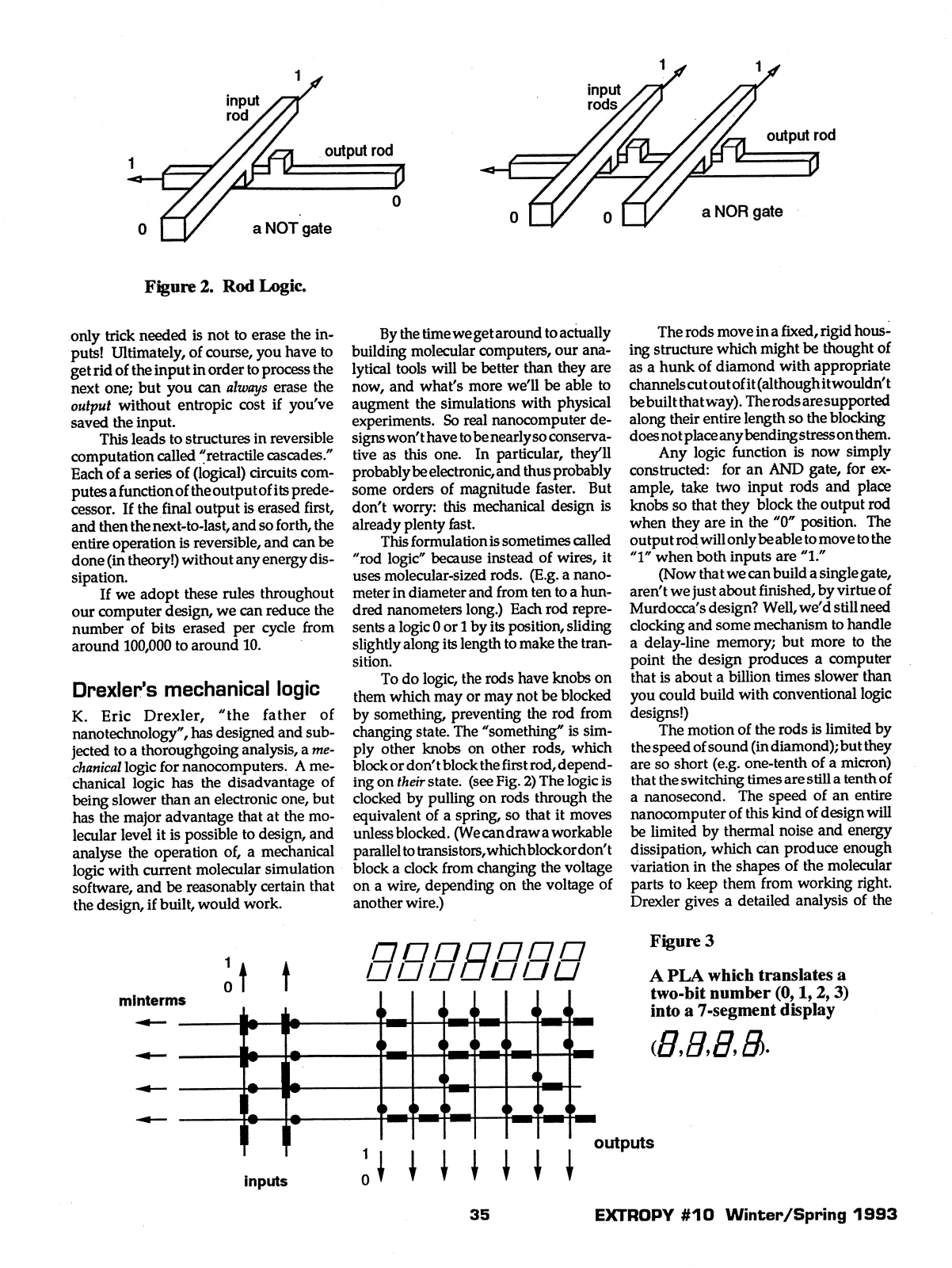
Figure 2. Rod Logic.

only trick needed is not to erase the inputs! Ultimately, of course, you have to get rid of the input in order to process the next one; but you can always erase the output without entropic cost if you’ve saved the input.

This leads to structures in reversible computation called “retractile cascades.” Each of a series of (logical) circuits computes a function of the output of its predecessor. If the final output is erased first, and then the next-to-last, and so forth, the entire operation is reversible, and can be done (in theory!) without any energy dissipation.

If we adopt these rules throughout our computer design, we can reduce the number of bits erased per cycle from around 100,000 to around 10.

Drexler’s mechanical logic

K. Eric Drexler, “the father of nanotechnology”, has designed and subjected to a thoroughgoing analysis, a mechanical logic for nanocomputers. A mechanical logic has the disadvantage of being slower than an electronic one, but has the major advantage that at the molecular level it is possible to design, and analyse the operation of, a mechanical logic with current molecular simulation software, and be reasonably certain that the design, if built, would work.

By the time we get around to actually building molecular computers, our analytical tools will be better than they are now, and what’s more we’ll be able to augment the simulations with physical experiments. So real nanocomputer designs won’t have to be nearly so conservative as this one. In particular, they’ll probably be electronic, and thus probably some orders of magnitude faster. But don’t worry: this mechanical design is already plenty fast.

This formulation is sometimes called “rod logic” because instead of wires, it uses molecular-sized rods. (E.g. a nanometer in diameter and from ten to a hundred nanometers long.) Each rod represents a logic 0 or 1 by its position, sliding slightly along its length to make the transition.

To do logic, the rods have knobs on them which may or may not be blocked by something, preventing the rod from changing state. The “something” is simply other knobs on other rods, which block or don’t block the first rod, depending on their state. (see Fig. 2) The logic is clocked by pulling on rods through the equivalent of a spring, so that it moves unless blocked. (We can draw a workable parallel to transistors, which block or don’t block a clock from changing the voltage on a wire, depending on the voltage of another wire.)

The rods move in a fixed, rigid housing structure which might be thought of as a hunk of diamond with appropriate channels cut out of it (although it wouldn’t be built that way). The rods are supported along their entire length so the blocking does not place any bending stress on them.

Any logic function is now simply constructed: for an AND gate, for example, take two input rods and place knobs so that they block the output rod when they are in the “0” position. The output rod will only be able to move to the “1” when both inputs are “1.”

(Now that we can build a single gate, aren’t we just about finished, by virtue of Murdocca’s design? Well, we’d still need clocking and some mechanism to handle a delay-line memory; but more to the point the design produces a computer that is about a billion times slower than you could build with conventional logic designs!)

The motion of the rods is limited by the speed of sound (in diamond); but they are so short (e.g. one-tenth of a micron) that the switching times are still a tenth of a nanosecond. The speed of an entire nanocomputer of this kind of design will be limited by thermal noise and energy dissipation, which can produce enough variation in the shapes of the molecular parts to keep them from working right. Drexler gives a detailed analysis of the

Figure 3

A PLA which translates a two-bit number (0, 1, 2, 3) into a 7-segment display

(0, 0, 0, 0).

EXTROPY #10 Winter/Spring 1993

sources of such error in Nanosystems (chapter 12). The energy dissipated per switch-

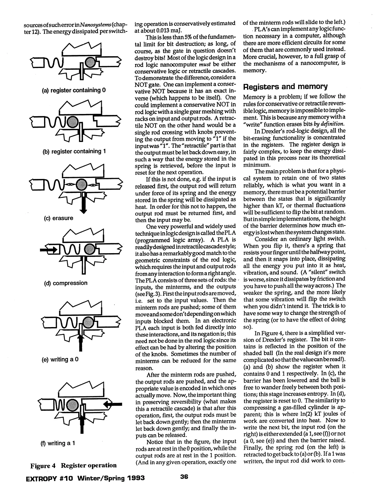
(a) register containing 0

(b) register containing 1

(d) compression

(e) writing a 0

(f) writing a 1

Figure 4 Register operation

ing operation is conservatively estimated at about 0.013 maJ.

This is less than 5% of the fundamental limit for bit destruction; as long, of course, as the gate in question doesn’t destroy bits! Most of the logic design in a rod logic nanocomputer must be either conservative logic or retractile cascades. To demonstrate the difference, consider a NOT gate. One can implement a conservative NOT because it has an exact inverse (which happens to be itself). One could implement a conservative NOT in rod logic with a single gear meshing with racks on input and output rods. A retractile NOT on the other hand would be a single rod crossing with knobs preventing the output from moving to “1” if the input was “1”. The “retractile” part is that the output must be let back down easy, in such a way that the energy stored in the spring is retrieved, before the input is reset for the next operation.

If this is not done, e.g. if the input is released first, the output rod will return under force of its spring and the energy stored in the spring will be dissipated as heat. In order for this not to happen, the output rod must be returned first, and then the input may be.

One very powerful and widely used technique in logic design is called the PLA (programmed logic array). A PLA is readily designed in retractile cascade style; it also has a remarkably good match to the geometric constraints of the rod logic, which requires the input and output rods from any interaction to form a right angle. The PLA consists of three sets of rods: the inputs, the minterms, and the outputs (see Fig. 3). First the input rods are moved, i.e. set to the input values. Then the minterm rods are pushed; some of them move and some don’t depending on which inputs blocked them. In an electronic PLA each input is both fed directly into these interactions, and its negation is; this need not be done in the rod logic since its effect can be had by altering the position of the knobs. Sometimes the number of minterms can be reduced for the same reason.

After the minterm rods are pushed, the output rods are pushed, and the appropriate value is encoded in which ones actually move. Now, the important thing in preserving reversibility (what makes this a retractile cascade) is that after this operation, first, the output rods must be let back down gently; then the minterms let back down gently; and finally the inputs can be released.

Notice that in the figure, the input rods are at rest in the 0 position, while the output rods are at rest in the 1 position. (And in any given operation, exactly one

of the minterm rods will slide to the left.)

PLA’s can implement any logic function necessary in a computer, although there are more efficient circuits for some of them that are commonly used instead. More crucial, however, to a full grasp of the mechanisms of a nanocomputer, is memory.

Registers and memory

Memory is a problem; if we follow the rules for conservative or retractile reversible logic, memory is impossible to implement. This is because any memory with a “write” function erases bits by definition.

In Drexler’s rod-logic design, all the bit-erasing functionality is concentrated in the registers. The register design is fairly complex, to keep the energy dissipated in this process near its theoretical minimum.

The main problem is that for a physical system to retain one of two states reliably, which is what you want in a memory, there must be a potential barrier between the states that is significantly higher than kT, or thermal fluctuations will be sufficient to flip the bit at random. But in simple implementations, the height of the barrier determines how much energy is lost when the system changes state.

Consider an ordinary light switch. When you flip it, there’s a spring that resists your finger until the halfway point, and then it snaps into place, dissipating all the energy you put into it as heat, vibration, and sound. (A “silent” switch is worse, since it dissipates by friction and you have to push all the way across.) The weaker the spring, and the more likely that some vibration will flip the switch when you didn’t intend it. The trick is to have some way to change the strength of the spring (or to have the effect of doing so).

In Figure 4, there is a simplified version of Drexler’s register. The bit it contains is reflected in the position of the shaded ball (In the real design it’s more complicated so that the value can be read!). (a) and (b) show the register when it contains 0 and 1 respectively. In (c), the barrier has been lowered and the ball is free to wander freely between both positions; this stage increases entropy. In (d), the register is reset to 0. The similarity to compressing a gas-filled cylinder is apparent; this is where ln(2) kT joules of work are converted into heat. Now to write the next bit, the input rod (on the right) is either extended (a 1, see (f)) or not (a 0, see (e)) and then the barrier raised. Finally, the spring rod (on the left) is retracted to get back to (a) or (b). If a 1 was written, the input rod did work to com-

EXTROPY #10 Winter/Spring 1993

press the ball into the spring, but that energy can be retrieved when the spring rod is retracted. The mechanisms to do this are just the same as in the logic portions, e.g. having the rods mechanically coupled to a flywheel.

Registers like this which are going to be used to erase bits will tend to be located near heat sinks or coolant ducts; bit erasure is the largest component of power dissipation in the rod logic design. Memory can be implemented as lots of registers; registers occupy about 40 cubic nanometers per bit. Thus about 3 megabytes worth of registers fill a cubic micron. One would probably use register memory for cache, and use a mechanical tape system for main storage, however. The “tape” would be a long carbon chain with side groups that differed enough to be 1’s and 0’s. Since the whole computer is mechanical, the difference in speeds is not as bad as macroscopic tapes on electronic computers. Such a tape system might have a density in the neighborhood of a gigabyte per cubic micron. Access times for using a tape as a random access memory consist almost entirely of latency; if the length of individual tapes is kept to under 100 kbytes, this is in the 10’s of microseconds.

Motors

In order to drive all this mechanical logic we need a motor of some kind; Drexler has designed an electric motor which is nothing short of amazing. (Clearly this is of import well beyond computers.) The reason is that the scaling laws for power density are in our favor as we go down toward the nanometer realm. At macroscopic sizes, almost all electric motors are electromagnetic; at nano scales, they will be electrostatic. The motor is essentially a van de Graff generator run in reverse (but it works just fine as a generator, as do some macroscopic electric motors). The power density of the motor is over 10^15 W/m^3; this corresponds to packing the power of a fanjet from a 747 into a cubic centimeter. (It’s not clear what you’d do with it if you did, though!)

Ultimately, the ability to make small, powerful motors is going to be more important for nanorobots than nanocomputers per se. The speed advantage of electronics over mechanical logic is almost certain to drive the descent into nanocomputer design.

Other logics for nanocomputers

Before going into other extensions of conventional digital logic, there is another

form of nanocomputer that may appear earlier for technological reasons. That’s the molecular biocomputer.

Imagine that a DNA molecule is a tape, upon which is written 2 bits of information per base pair (the DNA molecule is a long string of adenine-thymine and guanine-cytosine pairs). Imagine, in particular, this to be the tape of a Turing machine, which is represented by some humongous clump of special-purpose enzymes that reads the “tape,” changes state, replaces a base pair with a new one, and slides up and down the “tape.” If one could design the enzyme clump using conventional molecular biology techniques (and each of the individual functions it needs to do are done somewhere, somehow, by some natural enzyme) you’d have a molecular computer.

Other mechanical logics

Now, back to mechanical logic. Most macroscopic mechanical logic in the past has typically been based on rods that turned instead of sliding. It’s reasonable to assume that similar designs could be implemented at the nano scale.

Electronic logic

It’s clear that quantum mechanics allows for mechanisms that capture a single electron and hold it reliably in one place. After all, that’s what an atom is. Individual electrons doing specific, well-defined things under the laws of quantum mechanics, is what happens in typical chemical reactions. Clearly there is no basic physical law that prevents us from building nanocomputers that handle electrons as individual objects.

What is not so clear is how, specifically, they will work. Quantum mechanics is computationally very expensive to simulate, and intuitively harder to understand, than the essentially “physical object” models used in mechanical nanotechnology designs thus far. Indeed, the designs are typically larger and slower than they would have to be in reality, simply to avoid having to confront the analysis of quantum effects.

Ultimately, however, nanotechnologists will be “quantum mechanics.” Computers based on quantum effects will be even smaller, more efficient, and much faster than mechanical ones of the type presented above. They will use much the same logical structure: it’s quite possible to design retractile cascades even in conventional transistors (where it’s an extension of techniques called “dry switching” in power electronics and “hot clocks” in VLSI design).

There are schemes, with some mathematical plausibility, to harness quantum state superposition for implicit parallel processing. In my humble opinion, these will require some conceptual breakthrough (or at the very least, significant experimental clarification) about the phenomenon of the collapse of the Schroedinger wavefunction before they can be harnessed by a buildable device. Keep your fingers crossed!

Conclusion

Beyond certain rapidly approaching limits of size and speed, any computer must use logical reversibility to limit bit destruction. This is particularly true of nanocomputers with molecular-scale components, which if designed according to standard current-day irreversible techniques, explode.

We can design nanocomputers today which we are virtually certain would work if constructed. They use mechanical parts that are more than one atom but less than ten atoms across in a typical short dimension. The parts move at rates of up to ten billion times per second; processors built that way could be expected to run at rates of 1000 MIPS. Such a processor, and a megabyte of very fast memory, would fit in a cubic micron (the size of a bacterium). A gigabyte of somewhat slower memory would fit in another cubic micron. A pile of ten thousand such computers would be just large enough to see with the naked eye.